A simplified model of the connectome
Following the thinking process of a “typical neuroscientist”, we construct the model with the following assumptions:
Signals pass in a stepwise manner from one neuron to another through the synapses. So target neurons multiple synaptic hops away are reached later than those one synaptic hop away.
Excitation and inhibition take the same time to propagate (that is, one step).
The activation of a neuron ranges from “not active at all” (0) to “somewhat active” (0~1), to “as active as it can be” (1).
Unlike a “typical neuroscientist”, we also make the following assumptions:
Neurons are “points”. That is, we disregard synapse location, ion channel composition, cable radius etc..
We disregard neuromodulation for now (unless you know what a specific instance of neuromodulation should do, in which case you could either model by modifying the connection weights, or ask me to incorporate some new features in the package (yy432[at]cam.ac.uk)).
With these assumptions, we construct the following model, aiming to provide “connectome-based hypotheses” for your circuit of interest:
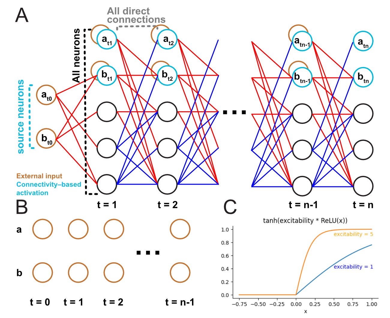
Panel A shows the implementation: all neurons are in each layer. Signed weights between adjacent layers are defined by the connectome. Each layer is therefore like a timepoint.
User can define a set of source neurons (blue/brown circles) which could be e.g. input to the central brain (sensory neurons, visual projection neurons, ascending neurons). External input is provided by activating the source neurons (brown / Panel B). The network is silent before any external input is fed in.
Panel C shows the activation function of each neuron: the (signed) weighted sum of the upstream neurons’ activity (x) is passed into a Rectified Linear Unit (ReLU()), scaled by excitability, and then passed into tanh(), to keep the activation of each neuron between 0 and 1.
An example implementation can be found here, which uses the MultilayeredNetwork().
Comparison with “effective connectivity”
Pros
nonlinearity (i.e. the curvature in panel C) - a bit more similar to real neurons;
users can see directly the response from a user-defined input pattern (panel B);
cheaper to compute than “effective connectivity”;
neuron activation don’t diminish with the increase in layers / time points, which does happen for “effective connectivity” calculation;
almost forces users to not cherry pick neurons/connections for interpretation in the densely-connected connectome.
Cons
a bit more complicated;
Plasticity
The connectivity in the connectome between some neurons, e.g. ring neurons and compass neurons, is only a scaffold for, instead of a direct reflection of, functional connectivity (Fisher et al. 2022). We therefore implemented (third-party-dependent) change in weights (“plasticity”), based also on the activation similarity of two groups of neurons (change_model_weights()).